Correlations between linguistic features are reflected in their geospatial patterning
Introducing the geo-typological Sandwich Conjecture
Uppsala, Konstanz, Manchester, IFISC
Roadmap
Background
typology \(\Rightarrow\) diachrony \(\Rightarrow\) typology
\(\Rightarrow\) Geo-spatial properties of linguistic features
Modelling distributions of individual features
- Rates of change & stability
- Our model (2021)
Modelling distributions of pairs of features
- Typological observations
- Word-order features & hypothesis testing
- Our model (2023)
- Spatial structure, entropy, and sandwichness
Empirical correlations between features
- Hypothesis evaluation
Outlook, etc.
Background
typology \(\Rightarrow\) diachrony \(\Rightarrow\) typology
- Question. Are you like your neighbours? Always? Why?
- There exists an intuition that neighbouring languages are likely to share various feature values, those that are very far apart less so.
- This intuition has two major underliers, both of which arguably lie in diachronic change:
- Phylogeny, vertical genetic descent — neighbours are more likely than non-neighbours to share a common origin;
- Contact, horizontal borrowing & transfer — neighbours are more likely to converge to one another over time than non-neighbours.
- Not trivial to separate out real-world results of one or the other.
- How do we tell apart contact-induced change, drift, independent parallel innovation, regular old inheritance? With difficulty or not at all?
- Question. Does this intuition about “being like your neighbours” depend on which features we’re talking about?
How different are different features in their susceptibility to (different kinds of?) change?
Background
Geo-spatial properties of linguistic features
Individual features show different kinds of spatial patterns.
Two randomly-chosen neighbours \(L_1\) and \(L_2\) are more likely to agree on basic word order than on def. art.
Heuristic: unstable features scatter, stable features cluster. (Question. Can stability be measured?)
Are features really independent? Do combinations of features have meaningful spatial distributions, too?
Background
Geo-spatial properties of linguistic features
A pair of features that might have a [linguistic] relationship, and a pair that probably doesn’t.
Harder to “visually inspect” than the simple case (therefore motivating defining some kind of measure …)
Distribution of pair of underlyingly-related f. ≠ distribution of pair of underlyingly-independent f. (?)
Modelling distributions of individual features
Rates of change & stability
Heuristic: unstable features scatter, stable features cluster. Question. Can stability be measured?
- Beginning with the one-feature case: considered individually, different typological features change on different timescales.
- This has given rise to quite a bit of work on rate-of-change estimation, mostly in the typological tradition.
- E.g. Maslova (2004), Wichmann and Holman (2009), Greenhill, Atkinson, Meade, and Gray (2010), Dediu (2011), Dediu and Cysouw (2013), Greenhill et al. (2017).
- Also our own work: Kauhanen et al. (2021), on which more shortly.
- E.g. Maslova (2004), Wichmann and Holman (2009), Greenhill, Atkinson, Meade, and Gray (2010), Dediu (2011), Dediu and Cysouw (2013), Greenhill et al. (2017).
- This has given rise to quite a bit of work on rate-of-change estimation, mostly in the typological tradition.
- Many of these discard spatial interactions between contiguous languages.
- Heuristic of this kind of work: stable features are conserved within language families. For unstable features, there is within-family variation.
- Most of this work also suggests that the present-day global distribution of language types reflects a stationary state of this process.
Modelling distributions of individual features
Rates of change & stability
Heuristic: unstable features scatter, stable features cluster. Question. Can stability be measured?
‘Stability estimation’ usually discards spatial interactions between contiguous languages.
- Is this a good model of reality? Problem(s, of which we are most concerned with this one):
- Perhaps some features are more prone to spatial interactions than others? (and so discarding spatial info. distorts data).
- Susceptibility to (phylogenetic) change by descent mostly about L1; to change by contact mostly about L2. Question then becomes whether we think these are homogeneous across features …
- Eg. uninterpretable (syntactic!) features — systematically L2-difficult, irrespective of L1 content? (Hawkins & Hatori 2006; Tsimpli & Dimitrakopoulou 2007)
- Work arguing that ‘simplifying’ change emerges from wholesale L2 learning (Trudgill 2001, Walkden & Breitbarth 2019): vulnerability to simplifying change = vulnerability to spatial interactions?
- Susceptibility to (phylogenetic) change by descent mostly about L1; to change by contact mostly about L2. Question then becomes whether we think these are homogeneous across features …
- If we think that the cognitive abilities involved in contact situations/L2 learning are not the same as those involved in child language acquisition, then we should be suspicious of the idea that spatial interactions aren’t variable.
- Even worse if we think, as many do, that L2 learning involves some kind of proper subset of L1.
Modelling distributions of individual features
Rates of change & stability
Heuristic: unstable features scatter, stable features cluster. Question. Can stability be measured?
‘Stability estimation’ usually discards spatial interactions between contiguous languages.
- Our previous work (Kauhanen et al. 2021): a model of the evolution of single (uncorrelated) features on a spatial substrate.
- Based on a conjecture of Greenberg’s (1978): we should be able to capture the kind of variability in spatial patterning that we’ve described entirely in terms of ingress and egress probabilities.
- Greenbergian ingress & egress + spatial dynamic from the classical “voter model” for spatial interactions (see Castellano, Fortunato, & Loreto, 2009, for an overview).
- Key finding: the diachronic stability of a feature can be predicted from its synchronic geospatial distribution
- Stable features cluster in space, unstable features don’t.
- Model has two interacting processes, each with a certain probability of occurring at each timestep:
- vertical: flip feature value at some given rate
- horizontal: copy feature value from geographical neighbour
Modelling distributions of pairs of features
Typological observations
The story so far. (We think) spatial distributions of individual features emerge from properties that we can treat as inherent to each feature — probabilities of egress and ingress ⊆ parameter denoting overall feature stability.
- But, we have talked about ‘features’ as though they operate independently.
- Not very plausible for a number of reasons interesting to us all:
- long history of implicational universals that involve multiple typological features of this type
- general interest in the idea of surface properties of (l/L)anguage being structurally related to one another
- Not very plausible for a number of reasons interesting to us all:
- From our point of view, two key tasks arise:
- extend the model we describe to the case of non-independent features: do we make predictions about the distributions that arise in this case?
- empirically test whether ‘preferred’ and ‘dispreferred’ combinations of features have predictable geographies (in the real world)
Modelling distributions of pairs of features
Word-order features
Do combinations of features have associated geo-spatial patterning?
- Proof-of-concept empirical example for this talk: word order features as in WALS, Dryer (2013), etc.
- Well-known and well-established as a paradigmatic example of (typologists’) features of this type that are strongly interdependent — certain combinations of features are disproportionately likely to be over- or under-represented.
As, of course, in various of Greenberg’s (1968) universals …
“In declarative sentences with nominal subject and object, the dominant order is almost always one in which the subject precedes the object.”
“In languages with prepositions, the genitive almost always follows the governing noun, while in languages with postpositions it almost always precedes.”
“Languages with dominant VSO order are always prepositional.”
“With overwhelmingly greater than chance frequency, languages with normal SOV order are postpositional.”
“If a language has dominant SOV order and the genitive follows the governing noun, then the adjective likewise follows the noun.”
“All languages with dominant VSO order have SVO as an alternative or as the only alternative basic order.”
- And in the long history of work on head-directionality, harmony …
Modelling distributions of pairs of features
Word-order features
Do combinations of features have associated geo-spatial patterning?
- Head-directionality (taken as a composite property) is fairly phylogenetically stable. It is also a canonical example of typologists’ harmony (Dryer 1992): all head-complement order tends to match the order of V and O within a given language.
- Cases in which headedness-related properties don’t match phylogenetic predictions tend to be attributed in the literature to contact effects: Indic, which is more rigidly OV than predicted due to Dravidian contact (Ledgeway & Roberts 2017); Iranian, where Persian is prepositional, Adj-N, and has head-initial relative clauses, but retains OV order and pre-head quantifers (…etc…) plausibly due to Turkic (Harris & Campbell 1995).
- Obvious thought: can we claim that Persian headedness is messy because it can ‘see’ lots of OV? (Not a new idea.)
- Cases in which headedness-related properties don’t match phylogenetic predictions tend to be attributed in the literature to contact effects: Indic, which is more rigidly OV than predicted due to Dravidian contact (Ledgeway & Roberts 2017); Iranian, where Persian is prepositional, Adj-N, and has head-initial relative clauses, but retains OV order and pre-head quantifers (…etc…) plausibly due to Turkic (Harris & Campbell 1995).
Prediction. The environments of ‘dispreferred types’ are more varied than ‘default’.
Modelling distributions of pairs of features
Hypothesis testing
Do combinations of features have associated geo-spatial patterning?
Intuition. The stability of a dispreferred type can be enhanced in certain configurations of contact.
(Sandwich Conjecture) Dispreferred ‘types’ should tend to be surrounded by a greater variety of types than preferred ‘types’.
- How do we model and test this?
- Question. How do we measure the ‘variety’ of the ‘surroundings’ of a language?
- Further question. Is there a measure of the inherent correlatedness of individual features that it’s worth thinking about (data-up, rather than theory-down)?
Modelling distributions of pairs of features
Incorporating feature correlations into our model
- Old model has two types of language: 0 and 1 (NO feature, YES feature).
- If the object of analysis is a pair of features, then we have a model that contains four types of language: 00, 01, 10, 11.
- Suppose features A and B correlate:
| A = 1 | A = 0 | |
|---|---|---|
| B = 1 | preferred | dispreferred |
| B = 0 | dispreferred | preferred |
| VO | OV | |
|---|---|---|
| prepositions | preferred | dispreferred |
| postpositions | dispreferred | preferred |
— such that \(f(11) \approx f(00) \gg f(01) \approx f(10)\).
Solution. Make the transition rates for A (B) depend on the value of B (A).
- This gets (can be made to get) the typological frequency distributions right
- But so far no spatial structure!
- It turns out that by specifying suitable transition rate parameter values, the Sandwich Conjecture is predicted
- First though, need a measure of “sandwichness”
Modelling distributions of pairs of features
Neighbourhood entropy, \(H\)
- Entropy \(H\) (information-theoretic) measures surprisal.
- In our case, the more varied a lge’s spatial neighbourhood is, the more surprisal.
- Formally, define neighbourhood entropy for language \(i\) with neighbourhood \(\langle i \rangle\), for type set \(T = \{00, 01, 10, 11\}\):
\[ H(i) = - \sum_{t \in T} P(t, \langle i \rangle) \log P(t, \langle i \rangle) \quad \text{with} \quad P(t, \langle i \rangle) = \frac{1}{|\langle i \rangle|} \sum_{j \in \langle i \rangle} \delta_{j,t}. \]

Modelling distributions of pairs of features
Sandwichness, \(\Xi\)
- Let \(\overline H(t)\) stand for Mean Neighbourhood Entropy (MNE) of type \(t\), computed across all lges
- If Sandwich Conjecture holds, MNE should be
- high for dispreferred types (because they’re surrounded by many types)
- low for preferred types (because they’re mostly surrounded by their own type)
- Define
\[ \Xi = \overline H(01) + \overline H(10) - \overline H(11) - \overline H(00) \]
i.e. entropies of dispreferred types minus entropies of preferred types
- High \(\Xi\): support for Sandwich Conjecture
- Low \(\Xi\): no support
Modelling distributions of pairs of features
Interim position
Where are we now?
Reasonable to expect typological correlations to give rise to geospatial patterns (Sandwich Conjecture).
- This can be captured even in a very simple model of language interactions on a spatial substrate.
Does this hold empirically, too?
- How do we model and test this?
Question. How do we measure the ‘variety’ of the ‘surroundings’ of a language?We can do this!- Further question. Is there a measure of the inherent correlatedness of individual features within the data that it’s worth thinking about?
- Simple measure of empirical correlation between variables: \(\varphi\), which for two features \(f_1\), \(f_2\):
| \(f_1\) = 1 | \(f_1\) = 0 | |
|---|---|---|
| \(f_2\) = 1 | 12 | 3 |
| \(f_2\) = 0 | 4 | 27 |
For each pair of (real-world) variables, how do \(\Xi\) and \(\varphi\) relate?
Empirical correlations between features
Hypothesis evaluation
Reasonable to expect typological correlations to give rise to geospatial patterns (Sandwich Conjecture).
For each pair of (real-world) variables, how do \(\Xi\) and \(\varphi\) relate?
- Issue. What if one type is vastly overrepresented? If the frequencies of the different types are very dissimilar, then even a random distribution of types over languages is not guaranteed to give \(\Xi\) = 0 (more frequent types are more likely to be surrounded by themselves, so their neighbourhood entropies can be expected to be slightly lower).
- One brute-force solution: carry out a permutation test by repeatedly recalculating \(\Xi\) over randomly-generated sets of languages. This gives us an idea of what kinds of values of \(\Xi\) to expect under the assumption that types are just randomly “thrown” onto the set of languages (and then something against which to compare our empirical \(\Xi\)).
- Calculate \(\Xi\) over the original dataset (pair of WALS features).
- Permute \(s\), the function that assigns types to languages (i. e. generate a new world in which languages have randomly-selected feature values).
- Calculate \(\Xi\) for permuted world.
- Repeat 2. and 3. many times.
Empirical correlations between features
Hypothesis evaluation
Reasonable to expect typological correlations to give rise to geospatial patterns (Sandwich Conjecture).
For each pair of (real-world) variables, how do \(\Xi\) and \(\varphi\) relate?
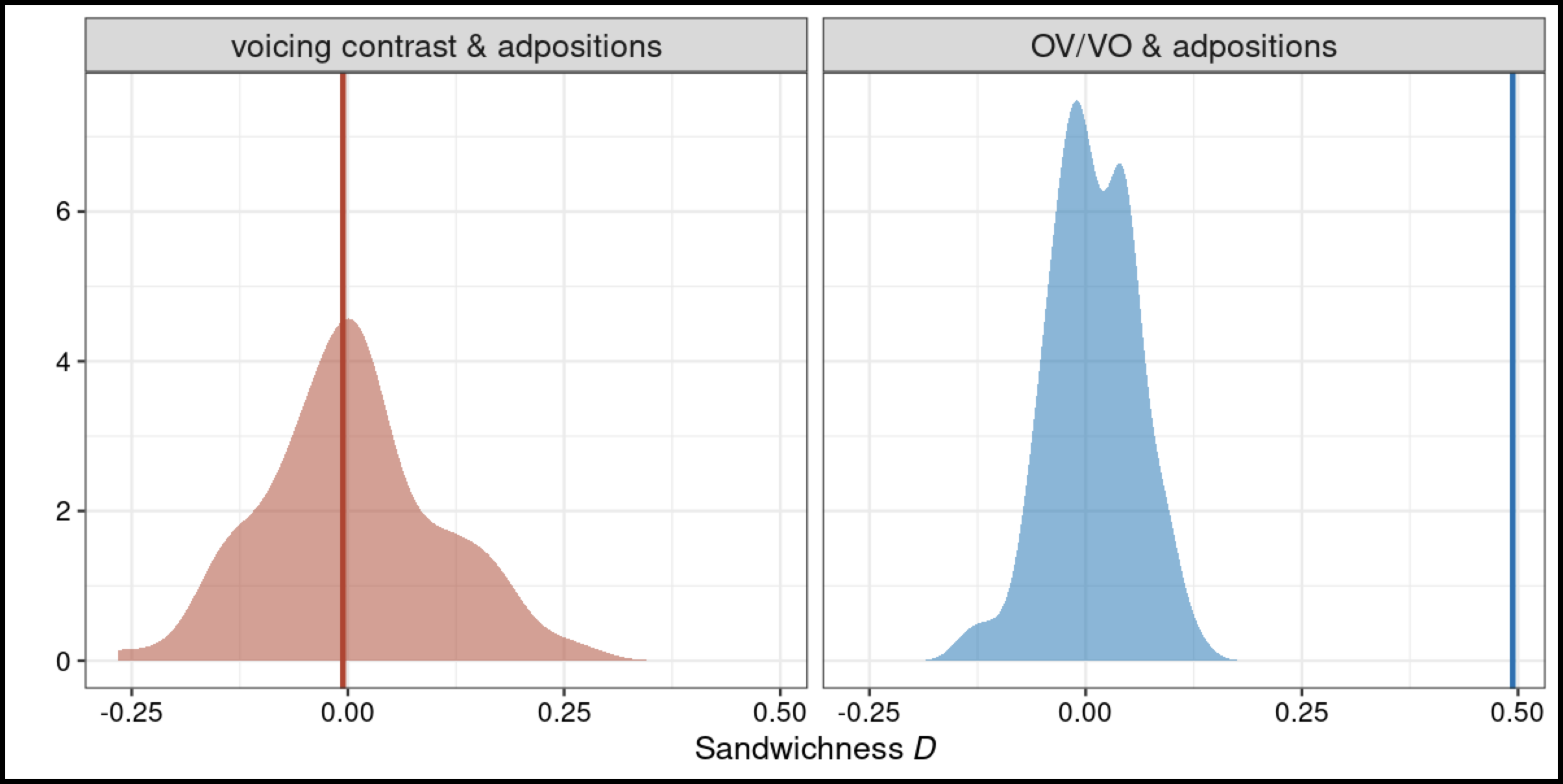
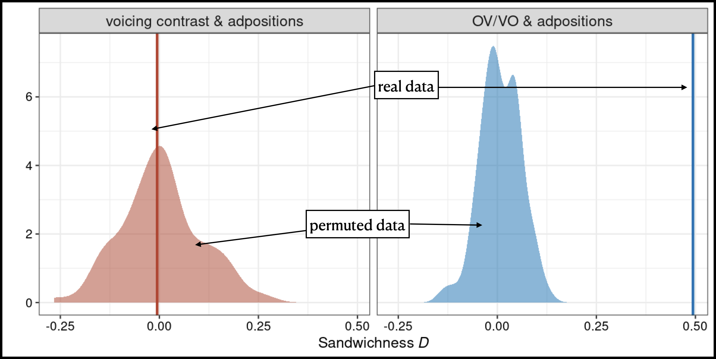
Quick illustration. The full result of this procedure for 3 WALS features: 83A, OV vs. VO, 85A, prepositions vs. postpositions, & 4A, obstruent voicing contrast.
Empirical correlations between features
Hypothesis evaluation
Reasonable to expect typological correlations to give rise to geospatial patterns (Sandwich Conjecture).
For each pair of (real-world) variables, how do \(\Xi\) and \(\varphi\) relate?
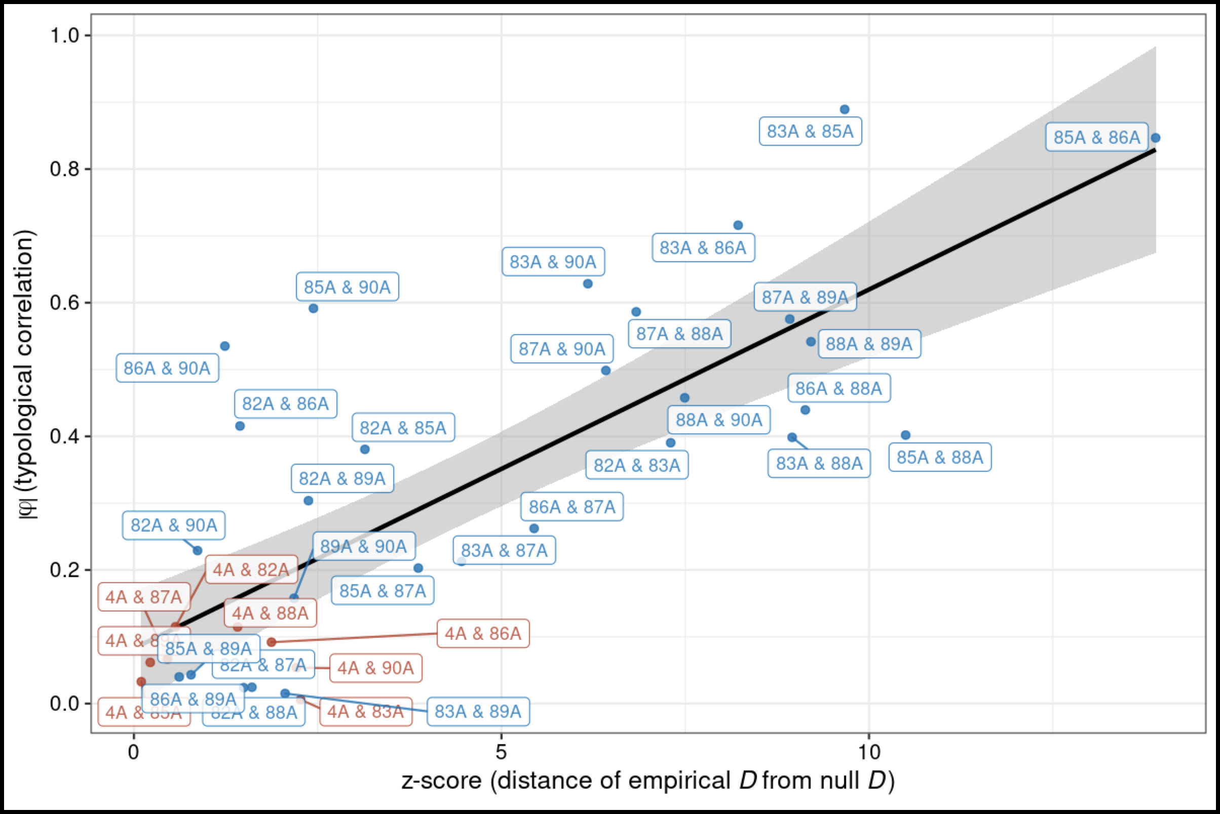
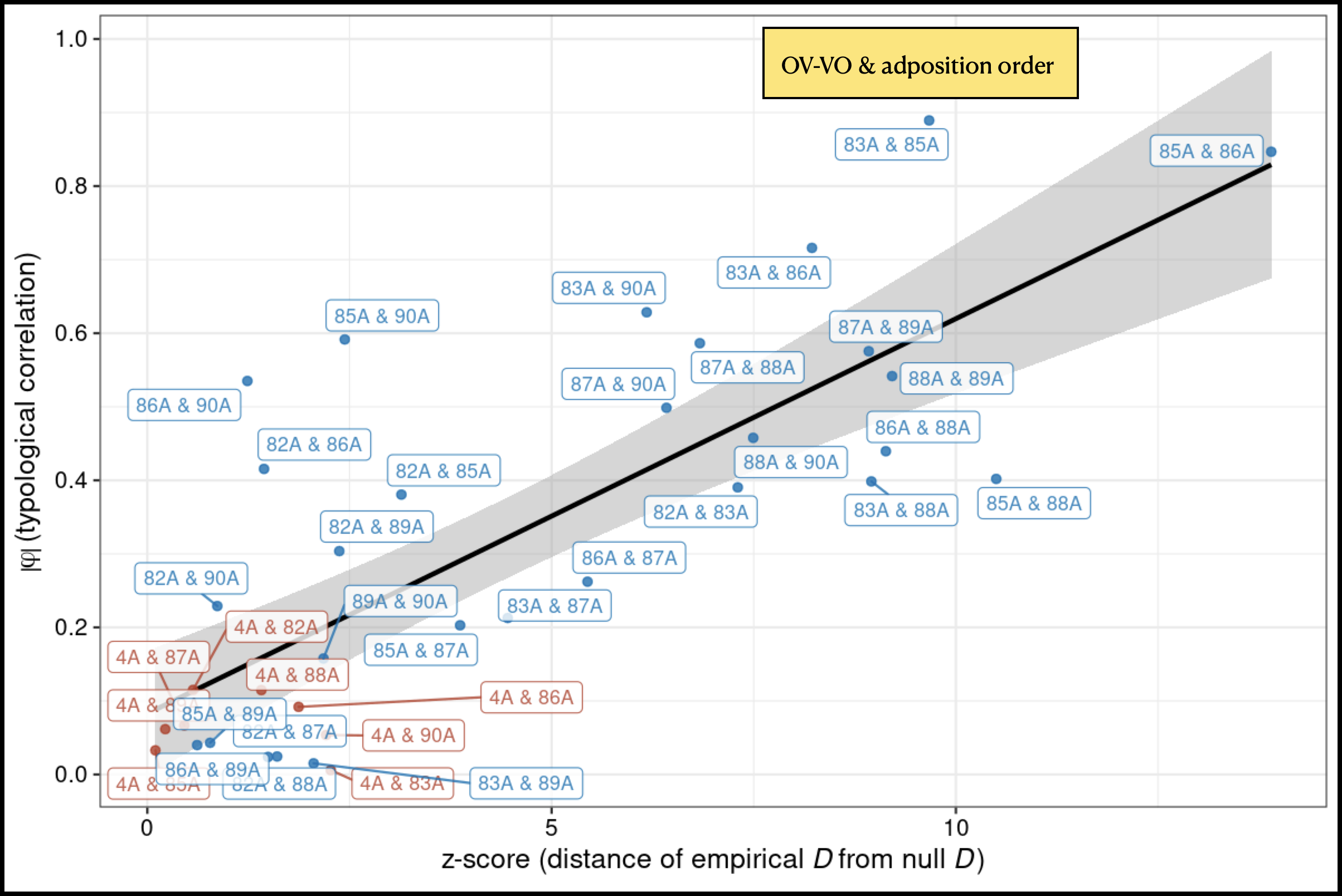
Larger illustration. The result of this procedure for all the WALS word-order features vs. 4A, obstruent voicing contrast, looking at z-score \(\Xi\) (empirical - null) only.
Conclusions & outlook
- Essential point of this talk. It’s nice to be able to frame typological facts that ‘everyone knows’ in ways that allow us to think about the emergent properties of simpler diachronic dynamics.
- Empirical spatial distributions have surprisingly predictable relationships to intuitions about actual linguistic properties and to hypotheses about ’how diachronic change is ordered‘.
- What we’d like to do next.
- A bit more robustness:
- Model analytics
- Proper model fits vis-à-vis data
- Bigger datasets (GramBank etc.)
- More domains (not just word order!)
- Spatial scales / granularity: is there a scale at which this stops holding? The individual? The small-scale speech community?
- A bit more robustness:
Thank you!
- For Kauhanen, Gopal, Galla, & Bermúdez-Otero (2021, Science Advances):
![]()
- For technical details, refs., etc. email us: gopal.deepthi@gmail.com + mail@hkauhanen.fi
